🔗 Github repository
🔗 Dataset Source 1
🔗 Dataset Source 2
Intro
The aim of this project is to analyze disease prevalence in the United States between 2019 and 2020 across different groups and measures. The project involves identifying patterns and trends in the data, building predictive models using Random Forest and Deep Neural Networking techniques, and exploring the factors that contribute to disease prevalence. The insights and predictions from this analysis can aid in decision-making processes related to public health interventions, resource allocation, and policy development.
Dataset
-
First Dataset: This dataset appears to contain information related to various health measures or indicators across different states and between 2019-2020.
-
Second Dataset: This dataset seems to provide information about population demographics, specifically focusing on age groups and racial categories within different states.
The project is built on two separate datasets: the first contains various estimates, chronic illness for various age groups, states, population, and health categories, whilst the second contains variables such as states, race, ten-year age groups, and population within percentage. Both datasets contain different types of information, with the first dataset focusing on health measures and the second dataset focusing on population demographics. They can potentially be used for analyzing health trends, studying population characteristics, or conducting research related to health and demographics.
Exploratory Data Analysis (EDA)
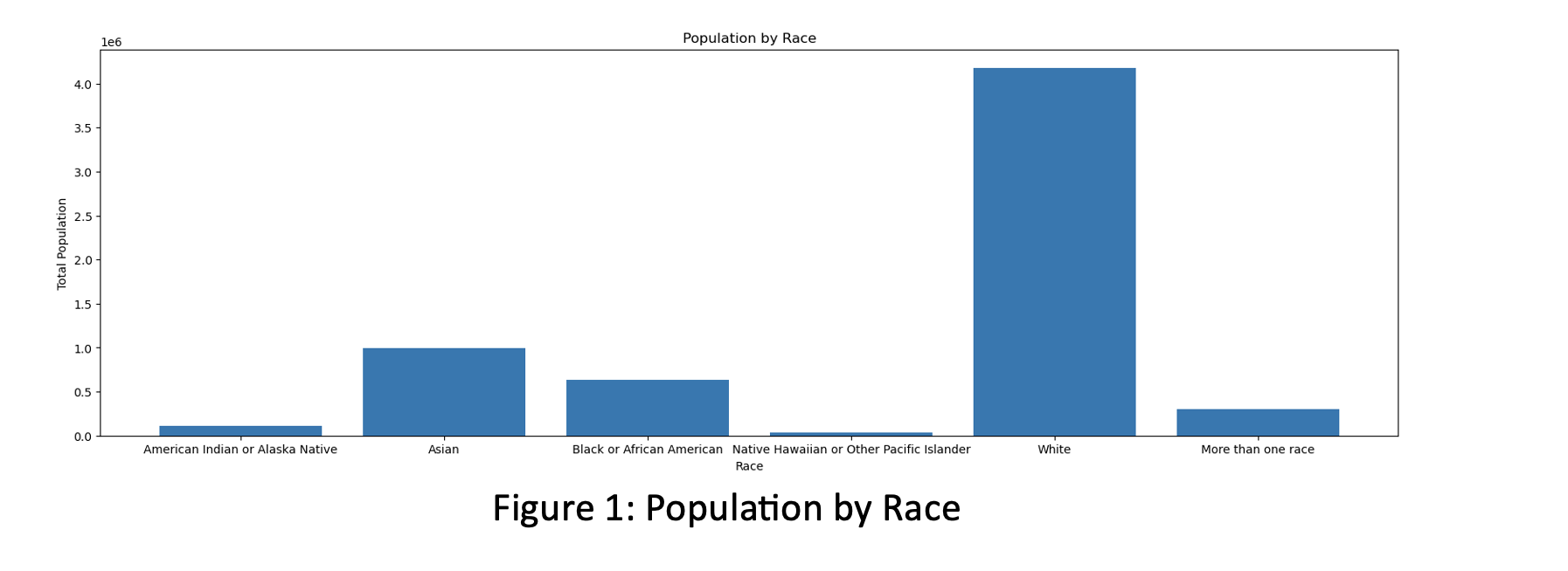 The bar chart for how total population is distributed over the races. Most of the people belong to White race; the Asian population is the second largest racial group. Black or African American people also represent significant portion of this population.
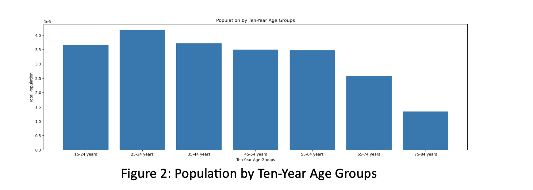 The bar chart for Population by Ten-Year Age Groups - how the people are distributed over the ages. The highest frequency is between 25- and 34-year-old groups. From 65 years age, this frequency goes down in graph.
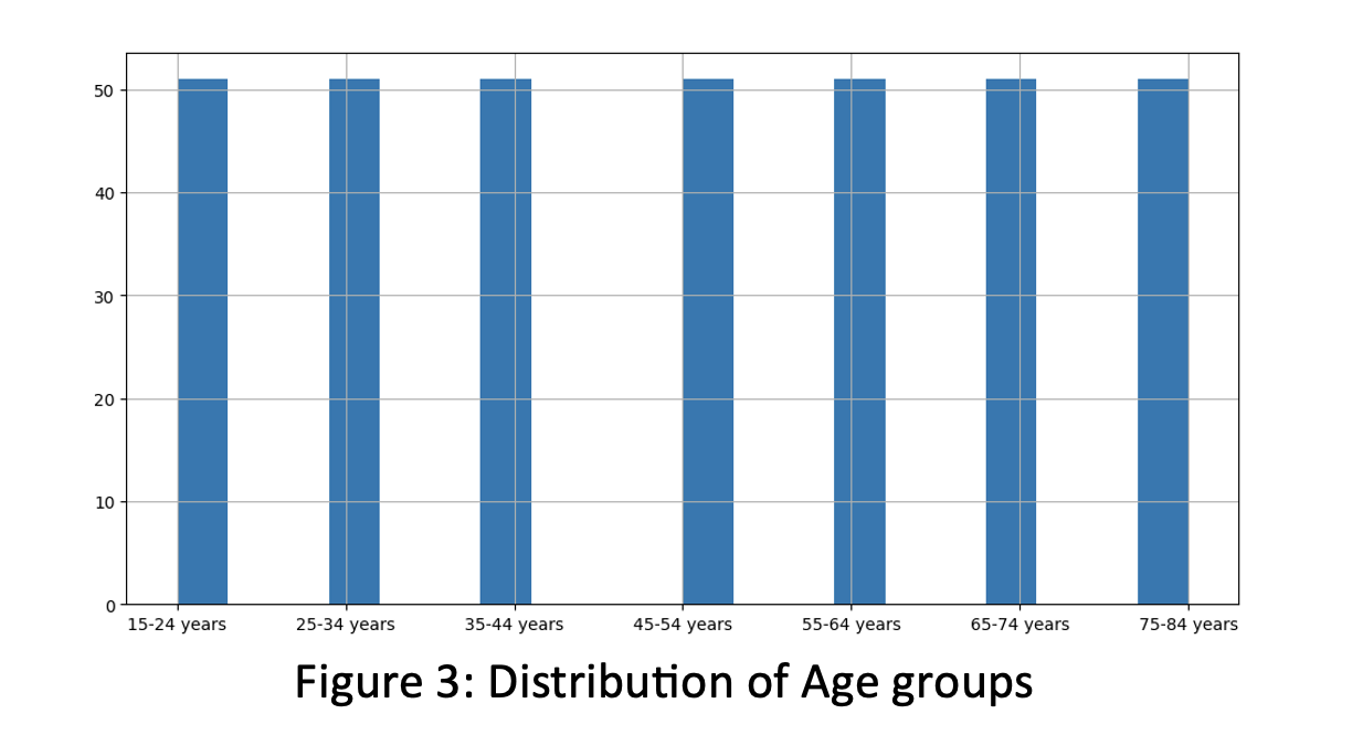 The histogram of Age groups to observe frequency of Ten-Year Age groups. It is determined that all age groups are equally distributed in the second dataset.
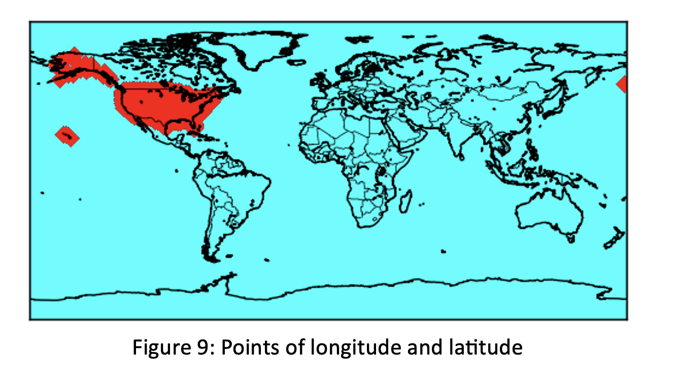 Using x and y as longitude and latitude coordinates which are splits of ‘Geolocation’ variable; we converted these coordinates into map scales and built map using marker as ‘D’ and Color as ‘red’.
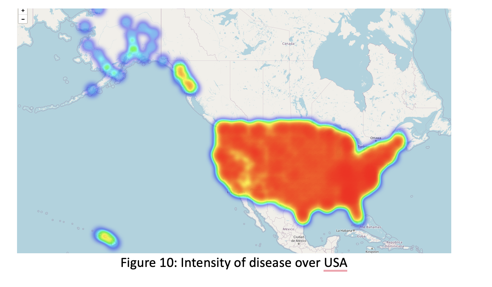 We could observe distribution of disease over USA within different colors which red shows high density while purple shows low density of disease. The map indicates that when east and middle states of the United States have high disease frequency, west states and around Alaska have low frequency.
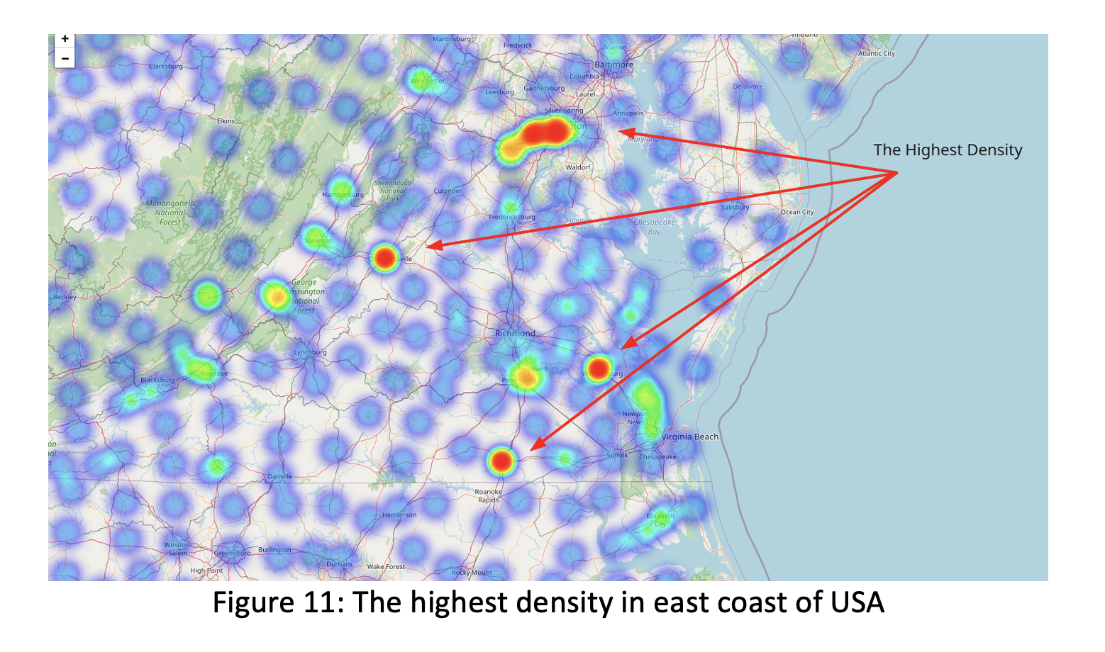 We highlighted some areas like Roanoke Rapids, Petersburg, Hopewell, Williamsburg- all these are in Virginia state, Manassas, Silver Spring, Towson which are Washington state areas as the highest density of illness records over the United States.
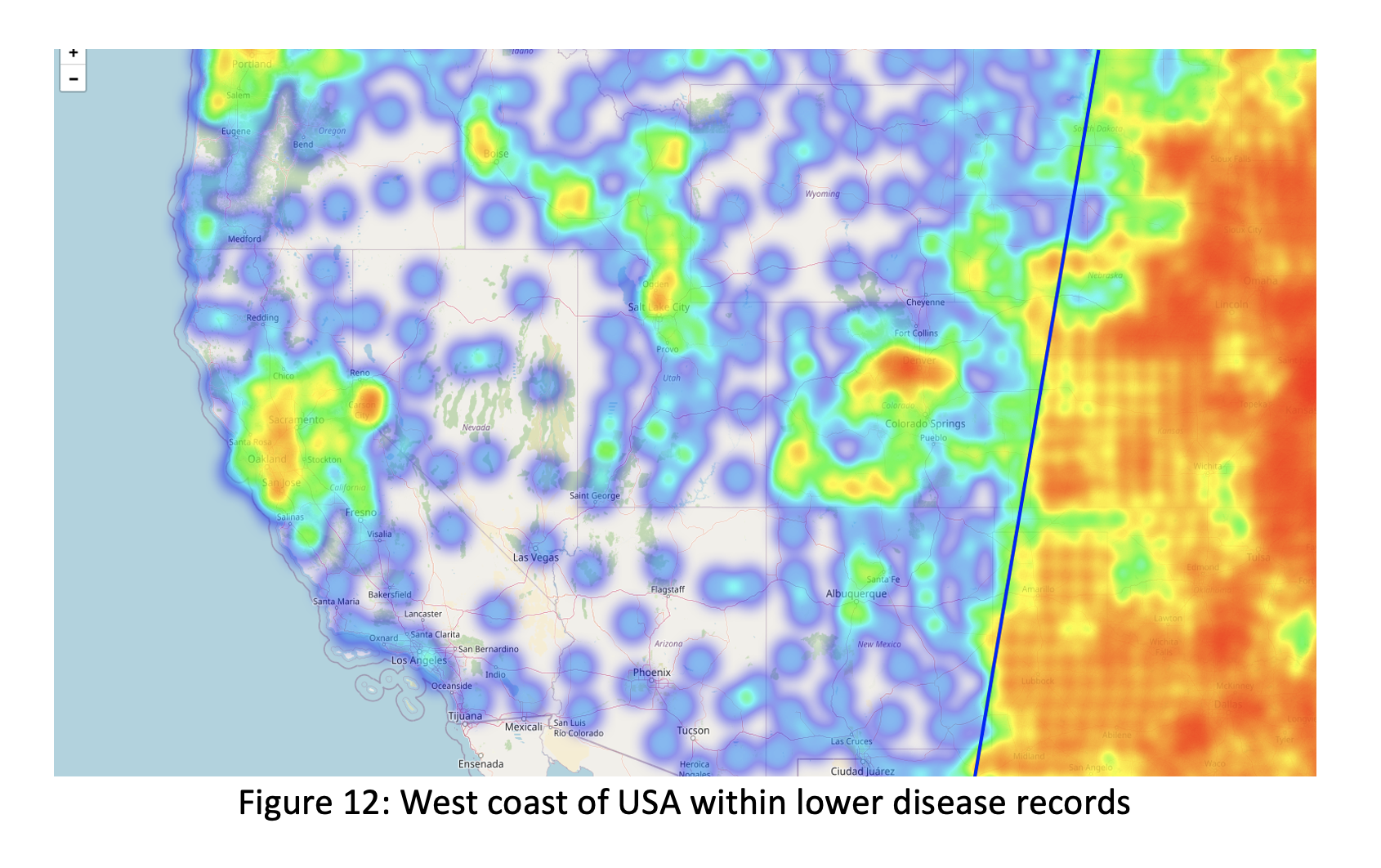 We identified that west coast areas have low density which purple color showed low disease records. Around these states high disease records have determined in some cities like Sacramento, San Jose, Salt Lake City, Colorado Springs, Utah, Bose (Idaho) which have colored with combination of green and yellow. Instead of having high population in California, we didn’t get high sickness over there.
Data Modelling
For applying DNN we uploaded torch, torch.nn packages on Python and converted our categorical variables (Category and Measure) into dummies. Then we converted the input features and target variable – ‘Data Value’ into PyTorch tensors and stores them. The len method returns the length of the dataset, and the getitem method allows indexing and retrieves a specific data sample from the dataset. The ‘MyModel’ class is a subclass of nn.Module, the base class for all neural network models in PyTorch. It defines the architecture of the model with three fully connected (linear) layers. The init method initializes the layers, and the forward method defines the forward pass of the model. The modified ‘MyModel’ class includes additional layers and the nn.LeakyReLU() activation function. Into architecture of model, two additional fully connected layers (fc4 and fc5) have been added, each with different input and output sizes. The nn.LeakyReLU() activation function is applied after each fully connected layer to introduce non-linearity in the model. After this process, we configurated parameters by set up the mode, dataset, device, data loader, loss function, and optimizer for training the neural network mode. The device variable is set based on the availability of CUDA (GPU). If CUDA is available, the model and dataset are moved to the GPU using model.to(device) and dataset.to(device). The dataset is explicitly moved to the device using dataset = dataset.to(device). This ensures that the dataset is also on the GPU if available, which is required for seamless training. The device variable is assigned with ‘cuda’ in the line device = torch.device(‘cuda’). The learning rate for the optimizer is set to lr=0.0005.
Feature Importance
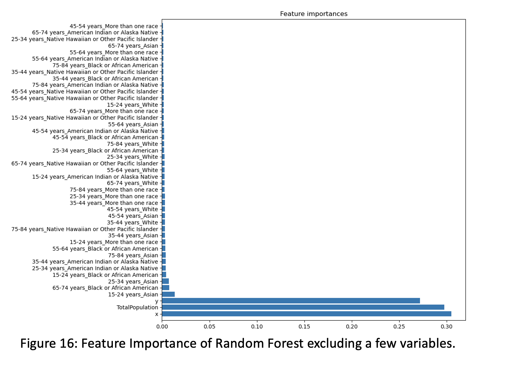 Races have very little impact on ‘Data Value’ variable. Only these races within different age group – 25-34 years Asian, 65-74 years Black or African American and 15-24 years Asian are more contributors in people who get illness. Additionally, we implemented AutoML model which checked all possible models and selected Random Forest Regressor as best model option which is great fact for our Random Forest model performance. In the final, for selecting the best predictive models for our dataset, we implemented Deep Neural Network which contains multiple successive layers of neurons- inputs to get output layer. We started to trained loop for the neural network model which iterates over the dataset for a specified number of epochs and performs forward and backward passes, updating the model’s parameters based on the calculated loss. The model consists of three fully connected layers with decreasing output sizes (128, 64, 1). The learning rate for the optimizer is set to lr=0.0005
The batch size was set to 128 and activation was ‘nn.ReLU()’. Furthermore, we accumulated the running loss for the current batch and evaluated the average loss for the epoch and kept those epoch loss in the list. The loss value is a measure of how well the model is performing on the training data. It quantifies the discrepancy between the predicted output of the model and the actual output. A lower loss value indicates better performance, as it suggests that the model’s predictions are closer to the true values. Our loss value in the epoch loss are fluctuating between 18-20 throughout training.
Conclusion
In this project, we aimed to gain meaningful insights from disease data and develop a predictive model to estimate disease prevalence. We utilized various models and techniques to achieve this objective. Based on these results, we could determine that our DNN model outperformed the Random Forest models in terms of predictive accuracy, achieving a lower MSE and higher R-squared value. This indicates that the DNN model captures the relationships between the variables more effectively, resulting in better predictions. From this model’s result and different analysis, we defined main factors to have diseases over the United States are Category, Measure, and location of disease. Considering those, decision-makers can make informed choices to address public health challenges effectively. The insights gained from our project and the predictive models developed can have significant implications for public health interventions, resource allocation, and policy development. By understanding the relationships between variables and accurately estimating disease prevalence, decision-makers can make informed choices to address public health challenges effectively. It is important to note that the accuracy and performance of our models are based on the available data and the specific features used. Further research, data refinement, and model optimization may be necessary to improve the accuracy and generalizability of the predictive models in real-world scenarios.
